This content originally appeared on Level Up Coding – Medium and was authored by Alexander Korostin

Motivation
Pathfinding is the process of finding an efficient route between two points in a system, whether it’s a game map, a road network, or even a sequence of currency trades. It’s not just about getting from A to B — it’s about doing it optimally, based on goals like shortest distance, fastest time, least fuel, or highest profit. Most pathfinding problems are modeled as graphs, where locations or states are nodes, and possible moves or actions are edges with associated costs or values.
But here’s the catch: real-world systems can’t just rely on basic algorithms like Dijkstra’s out of the box. While Dijkstra’s algorithm guarantees the shortest path in a graph with non-negative edge weights, it scales poorly. On a road network with 100,000 nodes, Dijkstra might explore tens of thousands of nodes to answer a single query. Now scale that to the real world: Google Maps must route across over 20 million road segments, covering hundreds of millions of intersections globally, and respond to billions of route requests per day, often returning results in under 100 milliseconds. A naïve implementation would be orders of magnitude too slow.
To make these systems viable, engineers use advanced algorithms like A* with domain-specific heuristics, Contraction Hierarchies, Customizable Route Planning, and preprocessed graph representations. For example, Contraction Hierarchies can answer queries 1000 times faster than Dijkstra’s algorithm on large road networks by precomputing shortcuts. Similarly, in games, algorithms like Jump Point Search and Hierarchical A* reduce the number of nodes explored by over 90% compared to classic approaches, which is crucial when hundreds of NPCs need to pathfind simultaneously at 60 frames per second.
Simply put, without decades of progress in pathfinding algorithms and optimization techniques, applications like Google Maps, Uber, or modern real-time strategy games would not be possible. They depend on highly tuned, scalable, and adaptive solutions that go far beyond textbook examples.
Classic Pathfinding Algorithms
Before we explore more advanced or domain-specific approaches, it’s important to revisit the foundational pathfinding algorithms. These classics still serve as the basis for many modern techniques.
Dijkstra
Dijkstra’s algorithm solves the single-source shortest path problem on graphs with non-negative edge weights. It explores nodes in order of increasing distance from the source, using a priority queue to always expand the least-cost node first. It guarantees the shortest path from the start node to all others. This makes it a good fit for applications like small road maps or board games where performance is not critical. However, its runtime — O((V + E) log V) with a binary heap — can become a bottleneck for larger graphs. The algorithm visits many unnecessary nodes when the target is known and far from the source, which is common in real-world scenarios. Here’s a basic version in Python:
import heapq

def dijkstra(graph, start):
    dist = {node: float('inf') for node in graph}
    dist[start] = 0
    queue = [(0, start)]

    while queue:
        cost, current = heapq.heappop(queue)
        if cost > dist[current]:
            continue
        for neighbor, weight in graph[current]:
            new_cost = cost + weight
            if new_cost < dist[neighbor]:
                dist[neighbor] = new_cost
                heapq.heappush(queue, (new_cost, neighbor))

    return dist
A*
A* (A-Star) is a modification of Dijkstra’s algorithm that uses a heuristic to guide the search toward the goal. It adds a priority function f(n) = g(n) + h(n), where g(n) is the cost from the start to node n, and h(n) is a heuristic estimate of the remaining distance to the goal. If the heuristic is admissible (never overestimates), A* is both optimal and often much faster than Dijkstra. The choice of heuristic depends on the domain: Manhattan distance for 2D grids, Euclidean for continuous space, and Haversine for geographic coordinates. A* is widely used in games for character navigation, and in maps for turn-by-turn routing. With a good heuristic, the number of visited nodes can drop by an order of magnitude. A simple implementation looks like this:
import heapq

def astar(graph, start, goal, heuristic):
    open_set = [(0, start)]
    g = {start: 0}
    came_from = {}

    while open_set:
        _, current = heapq.heappop(open_set)
        if current == goal:
            return reconstruct_path(came_from, current)
        for neighbor, cost in graph[current]:
            tentative_g = g[current] + cost
            if tentative_g < g.get(neighbor, float('inf')):
                came_from[neighbor] = current
                g[neighbor] = tentative_g
                f = tentative_g + heuristic(neighbor, goal)
                heapq.heappush(open_set, (f, neighbor))

    return None

def reconstruct_path(came_from, current):
    path = [current]
    while current in came_from:
        current = came_from[current]
        path.append(current)
    return path[::-1]
BFS
Breadth-First Search is the simplest of the bunch. It explores all neighbors at the current depth before moving to the next level, making it ideal for finding shortest paths in unweighted graphs. For example, it works well in puzzle solvers, mazes, or 2D tile-based maps where all moves have equal cost. It guarantees optimality in such cases, and runs in O(V + E) time. Here’s a minimal BFS that returns the shortest path:
from collections import deque

def bfs(graph, start, goal):
    queue = deque([start])
    visited = {start}
    came_from = {}

    while queue:
        current = queue.popleft()
        if current == goal:
            return reconstruct_path(came_from, current)
        for neighbor in graph[current]:
            if neighbor not in visited:
                visited.add(neighbor)
                came_from[neighbor] = current
                queue.append(neighbor)

    return None
DFS
Depth-First Search, in contrast, dives as deep as possible before backtracking. While not suitable for finding shortest paths, it’s useful in specific tasks like detecting connectivity or exploring all reachable nodes. In pathfinding, DFS is rarely used directly, but often plays a supporting role in graph analysis or pruning search spaces. Both iterative and recursive versions exist, but for completeness, here’s a concise recursive one:
def dfs(graph, start, visited=None):
    if visited is None:
        visited = set()
    visited.add(start)
    for neighbor in graph[start]:
        if neighbor not in visited:
            dfs(graph, neighbor, visited)
    return visited
These algorithms are the building blocks. Their limitations — especially in terms of scalability — are exactly what motivates the optimizations and hybrid techniques used in modern real-time systems.
Optimizations and Variants
Classic algorithms like Dijkstra’s and A* are powerful, but they can become inefficient on large maps or in real-time systems with strict performance requirements. Over time, researchers and engineers have developed a range of optimizations and algorithmic variants that dramatically reduce search time and memory usage while preserving path optimality or at least producing acceptable approximations. These enhancements are often domain-specific but are invaluable in practice, especially in games and large-scale navigation systems.
Bidirectional Search
Bidirectional search is a powerful optimization technique that accelerates shortest-path computations by simultaneously exploring from both the start and goal nodes. Instead of expanding nodes outward from just the source, it launches two searches: one forward from the start and one backward from the destination. These two frontiers expand toward each other until they meet somewhere in the middle. Once a common node is discovered in both directions, the shortest path can be reconstructed by combining the two partial paths. The key idea is that each search only needs to go approximately halfway, which leads to significant savings in both time and memory.
In an ideal scenario — such as a uniform graph (a graph where all edges have the same weight or cost) with a high branching factor (the average number of neighbors or successors each node has in a graph) — this technique can reduce the number of explored nodes from O(b^d) to O(b^(d/2)), where b is the average branching factor and d is the distance (in edges) between the start and goal. This exponential reduction is why bidirectional search is widely used in routing engines and navigation systems when the target node is known in advance.
While conceptually simple, bidirectional search introduces implementation challenges. Most importantly, the two searches must use compatible logic. In unweighted or uniformly weighted graphs, it’s common to use Breadth-First Search (BFS) in both directions. In weighted graphs, Dijkstra’s algorithm must be run in both directions using the same edge weights; however, the backward search must explore the graph with reversed edges unless the graph is undirected.
Another subtle issue is meeting point detection. It’s not enough for the front and back searches to simply visit the same node. We must identify the meeting point that minimizes the total cost of the combined path. To handle this correctly in weighted graphs, we typically maintain two cost maps: one from the forward search and one from the backward search. When a node appears in both, we compute the sum of forward and backward costs and track the minimal such total.
Here’s a practical Python implementation for unweighted graphs using BFS in both directions. The graph is represented as a dictionary mapping nodes to neighbor lists. This version returns the shortest path from start to goal as a list of nodes:
from collections import deque

def bidirectional_bfs(graph, start, goal):
    if start == goal:
        return [start]

    front_queue = deque([start])
    back_queue = deque([goal])

    front_parents = {start: None}
    back_parents = {goal: None}

    while front_queue and back_queue:
        meet_node = _expand_front(graph, front_queue, front_parents, back_parents)
        if meet_node:
            return _build_path(front_parents, back_parents, meet_node)

        meet_node = _expand_front(graph, back_queue, back_parents, front_parents)
        if meet_node:
            return _build_path(front_parents, back_parents, meet_node)

    return None  # No path found

def _expand_front(graph, queue, this_parents, other_parents):
    current = queue.popleft()
    for neighbor in graph.get(current, []):
        if neighbor not in this_parents:
            this_parents[neighbor] = current
            queue.append(neighbor)
            if neighbor in other_parents:
                return neighbor
    return None

def _build_path(front_parents, back_parents, meeting_point):
    path = []
    # build path from start to meeting_point
    node = meeting_point
    while node is not None:
        path.append(node)
        node = front_parents[node]
    path.reverse()
    # append path from meeting_point to goal
    node = back_parents[meeting_point]
    while node is not None:
        path.append(node)
        node = back_parents[node]
    return path
Jump Point Search
Jump Point Search (JPS) is an optimization technique designed specifically to speed up A* search on uniform-cost grids, commonly used in tile-based games and grid maps. Traditional A* expands many nodes step-by-step in all possible directions, which can be inefficient and redundant due to symmetrical paths — multiple sequences of moves leading to the same location with the same cost. JPS eliminates this redundancy by “jumping” over large stretches of nodes in straight lines until it reaches important points, called jump points, where the path must change direction or where forced neighbors exist.
The key insight behind JPS is that on uniform grids, many intermediate nodes can be skipped without missing the optimal path. Instead of expanding every neighbor, the algorithm recursively moves forward in a direction until it encounters a node that either: is the goal, has forced neighbors (neighbors that must be checked due to obstacles), or is a turning point. These nodes become the “jump points” and serve as the successors in the search. This pruning dramatically reduces the number of nodes evaluated — often by more than 90% — and speeds up pathfinding significantly while still guaranteeing optimal paths on grids with uniform movement cost.
JPS works on both 4-connected grids (up, down, left, right) and 8-connected grids (including diagonals). Unlike simple A*, it requires a specialized successor generation step but otherwise integrates with A*’s standard priority queue and cost calculations:
import heapq

def jump_point_search(start, goal, grid):
    open_list = []
    heapq.heappush(open_list, (0, start))  # (f_score, node)

    came_from = {}
    g_score = {start: 0}

    while open_list:
        _, current = heapq.heappop(open_list)

        if current == goal:
            return reconstruct_path(came_from, current)

        # prune_directions() is an application-specific function which
        # determines allowed directions to search from the current node
        for dx, dy in prune_directions(current, came_from):
            # jump() returns the next jump point in the given direction, or None
            jump_point = jump(grid, current[0], current[1], dx, dy, goal)
            if jump_point:
                tentative_g = g_score[current] + distance(current, jump_point)
                if jump_point not in g_score or tentative_g < g_score[jump_point]:
                    g_score[jump_point] = tentative_g
                    f_score = tentative_g + heuristic(jump_point, goal)
                    heapq.heappush(open_list, (f_score, jump_point))
                    came_from[jump_point] = current

    return None  # No path found
Here’s a simplified Python-style pseudocode illustrating the core jump function that moves recursively in a given direction until it finds a jump point or hits an obstacle:
def jump(grid, x, y, dx, dy, goal):
    nx, ny = x + dx, y + dy
    if not is_walkable(grid, nx, ny):
        return None
    if (nx, ny) == goal:
        return (nx, ny)

    # check for forced neighbors: positions that require a turn due to obstacles
    if has_forced_neighbors(grid, nx, ny, dx, dy):
        return (nx, ny)

    # diagonal movement requires recursive checks along both axes
    if dx != 0 and dy != 0:
        if jump(grid, nx, ny, dx, 0, goal) or jump(grid, nx, ny, 0, dy, goal):
            return (nx, ny)

    return jump(grid, nx, ny, dx, dy, goal)
In this snippet, is_walkable checks if the next cell is traversable, and has_forced_neighbors identifies nodes where alternative routes are forced by obstacles nearby. The recursive calls allow JPS to identify jump points both along straight and diagonal paths.
By skipping large stretches of uniform-cost nodes, Jump Point Search provides a major speedup compared to standard A* on grids, making it a popular choice in game development where hundreds of pathfinding queries may run every frame.
Theta* and Any-Angle Pathfinding
In grid-based pathfinding, standard algorithms like A* or Jump Point Search often produce paths that zigzag or follow rigid grid edges. While optimal in terms of node cost, such paths aren’t necessarily optimal in continuous space — especially in games or robotics where movement isn’t restricted to grid directions. This is where Any-Angle Pathfinding comes in, offering smoother, more realistic trajectories by allowing the agent to cut corners when possible.
Theta* is a well-known any-angle pathfinding algorithm that extends A* by relaxing its parent-child relationship constraint. In A*, a node’s parent is always one of its adjacent neighbors. Theta*, however, allows a node to be directly connected to its grandparent or even more distant ancestors — as long as there’s an unobstructed line of sight between them. This means it can “see through” intermediate nodes and link directly to farther predecessors, forming more natural, straight-line segments.
The modification is simple but powerful. During node expansion, instead of always computing the cost from the current node, Theta* checks whether the parent of the current node has a clear line of sight to the successor. If so, it computes the cost as if the parent directly reached that successor. If not, it falls back to the traditional method.
Here’s a minimal pseudocode of the core idea in Theta*:
def theta_star(grid, start, goal):
    open_list = []
    heapq.heappush(open_list, (0, start))
    came_from = {start: start}
    g_score = {start: 0}

    while open_list:
        _, current = heapq.heappop(open_list)

        if current == goal:
            return reconstruct_path(came_from, current)

        for neighbor in neighbors(grid, current):
            parent = came_from[current]
            if line_of_sight(grid, parent, neighbor):
                tentative_g = g_score[parent] + distance(parent, neighbor)
                if neighbor not in g_score or tentative_g < g_score[neighbor]:
                    came_from[neighbor] = parent
                    g_score[neighbor] = tentative_g
                    f_score = tentative_g + heuristic(neighbor, goal)
                    heapq.heappush(open_list, (f_score, neighbor))
            else:
                tentative_g = g_score[current] + distance(current, neighbor)
                if neighbor not in g_score or tentative_g < g_score[neighbor]:
                    came_from[neighbor] = current
                    g_score[neighbor] = tentative_g
                    f_score = tentative_g + heuristic(neighbor, goal)
                    heapq.heappush(open_list, (f_score, neighbor))

    return None
The key function here is line_of_sight(grid, a, b), which returns True if a straight line from a to b does not cross any obstacle. This is typically implemented using Bresenham’s line algorithm or a similar raycasting method.
Theta* produces much shorter and more realistic paths in open terrain, and because it still uses a graph-based search, it preserves many of A*’s guarantees, including completeness and optimality under certain grid conditions.
Hierarchical Pathfinding A*
When dealing with massive maps — like those in real-time strategy games or open-world simulations — standard A* or even JPS can become computationally expensive. These algorithms search at the lowest level of granularity: individual tiles or cells. But in real-world navigation (human or AI), we usually think in terms of high-level plans (“go to the north exit of the city”) and only later figure out the low-level details (exact turns and steps).
Hierarchical Pathfinding mimics this behavior by dividing the map into regions and introducing an abstract representation of connectivity between them. Instead of planning an entire path on the fine grid, the algorithm first searches in the abstract space, then refines the result into detailed movements within each region. This hierarchical decomposition drastically reduces the number of nodes explored.
A popular algorithm based on this idea is Hierarchical Path-Finding A* (HPA*), which works in three phases. It begins by dividing the map into fixed-size clusters — for example, grouping tiles into 10×10 blocks. Within each block, the algorithm identifies entrance and exit points where movement between adjacent clusters is possible. These points define the abstract connectivity of the map, essentially forming a coarse graph where each node represents a point on the border of a cluster.
From there, the algorithm constructs an abstract graph composed of these entry and exit nodes. It precomputes the shortest paths between all relevant pairs of such points within each cluster using standard A*, storing the results. Once the graph is built, the algorithm plans a path not on the original grid but on the abstract graph instead. It searches through the high-level space, jumping from cluster border to cluster border, which significantly reduces the number of nodes considered.
After this high-level plan is found, the algorithm proceeds to refine it. For each segment of the abstract path — that is, for each pair of connected entry or exit points — it performs a localized, low-level A* search within the corresponding cluster to determine the actual tile-by-tile path. These detailed paths are stitched together to form a complete, executable route from start to goal.
Here’s an outline of how an HPA* style method works:
def hierarchical_pathfinding(start, goal, grid, cluster_size):
    clusters = partition_grid(grid, cluster_size)
    entrances = identify_entrances(clusters)
    abstract_graph = build_abstract_graph(clusters, entrances)

    start_entrance = nearest_entrance(start, entrances)
    goal_entrance = nearest_entrance(goal, entrances)

    abstract_path = a_star_abstract(abstract_graph, start_entrance, goal_entrance)

    full_path = []
    for a, b in pairwise(abstract_path):
        cluster_path = a_star(grid, a, b)  # low-level A* in each cluster
        full_path.extend(cluster_path[:-1])  # avoid duplicate nodes

    full_path.append(goal)  # ensure goal is included
    return full_path
The performance boost comes from this abstraction. On a 200×200 map, a regular search would need to examine up to 40,000 individual tiles. But if the map is divided into 10×10 clusters, the abstract graph might involve only a few hundred critical nodes. This reduction in search space translates to dramatic improvements in speed, especially in real-time environments where many agents request paths simultaneously.
Advanced and Domain-Specific Approaches
As pathfinding problems scale beyond grids and games into massive, real-world networks like road maps, railways, and logistics graphs, classic algorithms start to fall short. These domains demand not just speed, but also support for multiple criteria — like distance, travel time, toll costs, and even dynamic traffic. In such cases, purely online algorithms like A* or even Jump Point Search often aren’t fast enough, especially when real-time response is required across vast search spaces.
To address this, advanced pathfinding techniques rely heavily on preprocessing. By analyzing the structure of the network ahead of time and storing auxiliary data like shortcuts, landmarks, or region partitions, these algorithms shift much of the work offline. The result is dramatically faster queries at runtime — sometimes in milliseconds — even across graphs with millions of nodes.
Contraction Hierarchies
Contraction Hierarchies (CH) are a powerful preprocessing-based pathfinding technique designed for very large and sparse graphs, especially road networks. In such networks, the number of nodes can reach into the tens of millions, and naive shortest-path algorithms like Dijkstra’s become prohibitively slow. Contraction Hierarchies address this by adding shortcut edges to the graph during an offline preprocessing phase, allowing the query phase to run extremely fast — often in just a few milliseconds.
The core idea behind CH is deceptively simple: some nodes are more important than others for long-distance routing. For example, highways are more likely to appear in the middle of a cross-country route than tiny side streets. CH exploits this by assigning each node an importance and then removing (or “contracting”) less important nodes, while preserving shortest-path distances by inserting shortcut edges between their neighbors.
During preprocessing, nodes are contracted one by one in increasing order of importance. When a node v is contracted, the algorithm looks at all incoming edges (u → v) and outgoing edges (v → w), and determines whether it must insert a direct edge (u → w) that represents the shortest path through v. This process is repeated until all nodes are contracted. The result is a graph augmented with shortcuts that implicitly represent multi-hop paths via contracted nodes, but with no loss of correctness.
Once the preprocessing is done, shortest-path queries are extremely efficient. CH uses a bidirectional Dijkstra-like search, but restricted to only follow upward edges — edges going to more important nodes — in both forward and backward directions. The search meets somewhere in the middle, and because it’s navigating through a much smaller and higher-level skeleton of the graph, it finishes quickly.
Here is a simplified outline of the query phase in Python-style pseudocode:
def ch_query(graph, start, goal):
    forward_queue = PriorityQueue()
    backward_queue = PriorityQueue()
    forward_dist = {start: 0}
    backward_dist = {goal: 0}
    visited = set()

    forward_queue.push((0, start))
    backward_queue.push((0, goal))

    best = float('inf')

    while not forward_queue.empty() or not backward_queue.empty():
        best = min(best, relax_ch_edges(forward_queue, forward_dist, backward_dist, graph, visited, direction='up'))
        best = min(best, relax_ch_edges(backward_queue, backward_dist, forward_dist, graph, visited, direction='up'))

    return best
The key constraint in CH is that each direction only considers edges leading to more important nodes, keeping the search narrow and efficient. Thanks to the shortcut structure built during preprocessing, CH can skip over large sections of the graph in just a few hops, making it exceptionally fast for long-distance routing. However, this same structure becomes a liability for short-distance queries. When the source and target are close together, navigating the hierarchy and evaluating shortcut edges often introduces unnecessary overhead. In such cases, simpler local methods — like unidirectional Dijkstra — can be faster in practice.
ALT Algorithm
The ALT algorithm — short for A*, Landmarks, and Triangle Inequality — is a powerful variant of A* that significantly improves query performance on large-scale graphs like road networks. Before understanding how it works, it’s helpful to define the two mathematical ideas it builds on: landmarks and the triangle inequality.
A landmark is simply a node in the graph that serves as a fixed reference point. During a preprocessing phase, the algorithm computes and stores the shortest-path distances between all nodes and a selected set of these landmarks. These distances don’t change from one query to another, so they can be reused for fast distance estimates at query time.
The triangle inequality, a property of metric spaces, states that for any three points uuu, vvv, and lll, the direct distance from u to v is never greater than going from u to l and then from l to v. This inequality is the core of ALT’s heuristic.
With this in place, the ALT algorithm works as follows: in an offline preprocessing step, it selects a set of landmarks and computes shortest-path distances to and from each landmark for all nodes in the graph. At query time, these distances are used to estimate the shortest path from a current node to the goal. Instead of relying on spatial heuristics like Euclidean or geographic distance, ALT uses the triangle inequality to produce a tighter and more graph-accurate lower bound.
For a given node n, the heuristic used by A* becomes:
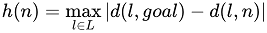
where L is the set of landmarks, and d(l, x) is the precomputed distance between landmark l and node x. Taking the maximum ensures we’re always using the tightest available lower bound among all landmarks.
This results in far more efficient searches. Instead of blindly exploring the graph, ALT pushes the search in directions that are likely to lead to the goal while safely pruning away large irrelevant regions. It still guarantees the shortest path but does so with far fewer node expansions than plain A*.
Here’s a simplified pseudocode of how ALT integrates into an A* search loop:
def alt_search(graph, start, goal, landmarks, dist_to_landmark, dist_from_landmark):
    open_list = []
    heapq.heappush(open_list, (0, start))
    came_from = {}
    g_score = {start: 0}

    def heuristic(n):
        return max(
            abs(dist_from_landmark[l][goal] - dist_from_landmark[l][n])
            for l in landmarks
        )

    while open_list:
        _, current = heapq.heappop(open_list)

        if current == goal:
            return reconstruct_path(came_from, current)

        for neighbor in graph.neighbors(current):
            tentative_g = g_score[current] + graph.cost(current, neighbor)
            if neighbor not in g_score or tentative_g < g_score[neighbor]:
                g_score[neighbor] = tentative_g
                f_score = tentative_g + heuristic(neighbor)
                heapq.heappush(open_list, (f_score, neighbor))
                came_from[neighbor] = current

    return None
The effectiveness of ALT depends on choosing good landmarks. Common strategies include selecting nodes at the edges or corners of the graph, nodes with high centrality, or farthest pairs. The more “strategic” the landmarks, the tighter the heuristic and the faster the query.
Customizable Route Planning and Multi-Level Dijkstra
Customizable Route Planning (CRP) is a state-of-the-art routing algorithm designed for systems that need both fast queries and the ability to quickly adapt to changing edge weights — such as live traffic updates, user preferences, or multi-criteria costs. It is especially well-suited for real-world applications like interactive map services, logistics platforms, and multimodal routing engines. The concept was originally introduced under the name CRP, but in modern systems like OSRM, it has evolved into a more scalable variant known as MLD (Multi-Level Dijkstra).
The core innovation behind CRP and MLD is to decouple topology from cost. This is done by splitting preprocessing into two clearly defined phases.
First, a metric-independent preprocessing step partitions the graph into nested clusters or “cells”. This phase doesn’t depend on travel time, distance, or any cost function — only the structure of the graph. It constructs a multi-level hierarchy of these partitions and identifies boundary nodes — the entry and exit points between cells. Because this step is independent of weights, it only needs to be performed once, even if the cost metric changes later.
The second phase is metric-dependent customization. Here, the algorithm computes shortcuts between all pairs of boundary nodes within each cell based on the current edge weights. This step is much faster than the full preprocessing and can be repeated on the fly when traffic conditions change or when a different cost metric is used (e.g., toll avoidance, EV charging efficiency). In practice, customization can complete in under a second on large-scale road networks.
When answering a query, CRP/MLD uses a multi-level Dijkstra search that hops across boundaries, exploring only those parts of the graph necessary to connect start and goal through the partition hierarchy. This drastically reduces the number of nodes expanded compared to classic Dijkstra or even A*, while still incorporating dynamic edge costs.
An (over)simplified flow might look like this:
# Phase 1: Metric-Independent Preprocessing (run once)
def preprocess_graph(graph):
    # Recursively partition the graph into cells at multiple levels
    levels = []
    current_level = graph
    while size(current_level) > threshold:
        cells = partition(current_level)  # e.g., via METIS or KaHIP
        boundary_nodes = identify_boundary_nodes(cells)
        levels.append((cells, boundary_nodes))
        current_level = build_abstract_graph(cells, boundary_nodes)
    return levels

# Phase 2: Metric-Dependent Customization (repeatable for new weights)
def customize_weights(levels, edge_weights):
    for cells, boundary_nodes in levels:
        for cell in cells:
            # For each pair of boundary nodes in cell, compute shortest path shortcuts
            shortcuts = compute_shortcuts(cell, boundary_nodes[cell], edge_weights)
            update_cell_with_shortcuts(cell, shortcuts)

# Phase 3: Query (per path request)
def query_path(levels, start, goal, edge_weights):
    # Initialize search structures on all levels
    open_sets = init_open_sets(levels)
    distances = init_distances(levels, start, goal)

    while not all_open_sets_empty(open_sets):
        # Perform a level-aware multi-directional Dijkstra step
        for level in reversed(levels):
            relax_edges(open_sets[level], distances, edge_weights, level)
        # Check for meeting point between forward and backward searches

    return reconstruct_path(distances, start, goal)
An important note here: The original CRP algorithm was patented by Microsoft, which limited its use in some commercial products without licensing. However, open-source systems like OSRM have adopted similar ideas under the name MLD, with algorithmic differences that avoid patent claims.
Afterword
Pathfinding might sound like a niche topic, but it’s actually behind a lot of tech we use every day — from getting directions on your phone to how game characters find their way around. Over the years, algorithms have gotten smarter and faster, evolving from simple stuff like Dijkstra’s to clever tricks like Contraction Hierarchies and Customizable Route Planning that handle massive maps and changing conditions with ease. And the field keeps moving forward with cool new ideas like AI-driven pathfinding and ways to adapt on the fly when things change. Whether you’re building a game, a mapping app, or just curious about how this all works, understanding these techniques can give you a real edge in making things faster, smoother, and smarter.
Pathfinding in Games and Geospatial Applications was originally published in Level Up Coding on Medium, where people are continuing the conversation by highlighting and responding to this story.
This content originally appeared on Level Up Coding – Medium and was authored by Alexander Korostin