A Practical Guide to Incremental Updates and Transfer Learning for Scalable New-Product Forecasting…

This content originally appeared on Level Up Coding – Medium and was authored by Satyajit Chaudhuri

A Practical Guide to Incremental Updates and Transfer Learning for Scalable New-Product Forecasting using MLForecast

Practical principles, code patterns, and decision rules for data scientists deploying new-product forecasts and incremental forecasts in production.

Forecasting demand is one of the few problems where science meets business head-on. Theoretical models, statistical assumptions, and machine learning architectures look compelling in notebooks — until they meet production systems with streaming data, new product launches, and evolving seasonality.

In the last few years, Nixtla’s MLForecast has quietly reshaped how researchers and data scientists handle time series forecasting at scale. Unlike traditional statistical approaches, MLForecast bridges the gap between machine learning feature engineering and forecasting principles, allowing tree-based models like LightGBM, XGBoost, and Random Forest to behave like robust time series forecasters — even across millions of series. A detailed walkthrough of this is available here.

The deeper question every data scientist asks when moving from experimentation to production is:

“Should we retrain the model every time new data arrives?”

This article answers that question — and then goes further. We show how Nixtla’s update() method and its transfer-learning approach together form the operational backbone of production-grade forecasting systems: fast enough for business cadence, principled enough for research, and auditable enough for enterprise adoption.

The article is organized into two complementary parts:

1. Incremental updates with update() — a production-first treatment of how to absorb fresh monthly observations without costly retraining. You’ll learn the API mechanics, why update() preserves model stability and latency, when it suffices, and when it must be paired with scheduled retraining or drift detection.
2. Transfer learning for new-product forecasting — a research-informed, practitioner-tested guide to pretraining global models and applying them zero- or few-shot to cold-start SKUs. We cover practical recipes (zero-shot, warm-start via update(), and light fine-tuning), business trade-offs, and how to combine human judgement with model outputs.

1. MLForecast — A Global Approach to Prediction

MLForecast is not just another forecasting library — it’s a meta-framework that converts tabular machine learning into scalable forecasting.

Unlike ARIMA or Prophet, which build individual models per series, MLForecast creates a global model that learns from patterns shared across all products, stores, or geographies.

At its core, it automates:

• Lag feature creation (y[t-1], y[t-2], …),
• Rolling statistics (mean, std, min, max),
• Date-based covariates (month, quarter, holiday, seasonality).

This makes models like LightGBM or XGBoost inherently capable of learning seasonality and temporal dependencies — without relying on hand-crafted transformations.

from mlforecast import MLForecast
from xgboost import XGBRegressor
from lightgbm import LGBMRegressor
from sklearn.ensemble import RandomForestRegressor

models = {
    'xgb': XGBRegressor(objective='reg:squarederror', n_estimators=200),
    'lgb': LGBMRegressor(n_estimators=200, verbosity=-1),
    'rf': RandomForestRegressor(n_estimators=200, n_jobs=-1)
}

fcst = MLForecast(
    models=models,
    freq='MS',
    lags=[1, 2, 3, 6, 12],
    date_features=['month', 'year']
)

fcst.fit(Y_df)  # Y_df = ['unique_id', 'ds', 'y']

Once trained, this global model forecasts every series in your dataset simultaneously — a powerful property when you have hundreds or thousands of SKUs.

2. Let's update() the Forecast

When your forecast system goes live, data doesn’t stop. Every month, new observations arrive — and decision-makers expect your forecasts to reflect reality immediately.

The naive solution is to retrain the model every time new data arrives.
But that’s computationally expensive, time-consuming, and operationally risky.

This is where MLForecast’s update() method becomes crucial.

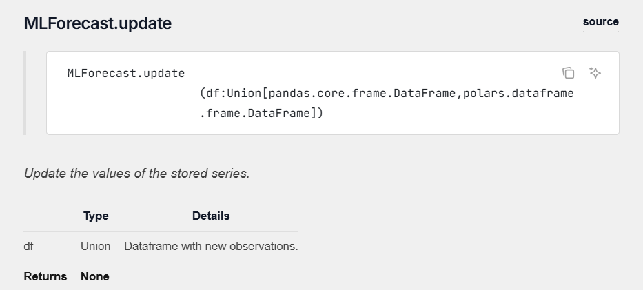
2.1 What update() Does!

The update() method allows your trained forecasting object to absorb new observations without retraining the underlying model. It simply extends the historical window for each series so that subsequent forecasts are generated using the most recent real values.

new_data = pd.DataFrame({
    'unique_id': ['prod_01', 'prod_02'],
    'ds': ['2025-10-01', '2025-10-01'],
    'y': [128.5, 92.1]
})

fcst.update(new_data)
preds = fcst.predict(h=3)

Behind the scenes:

• The new y values are appended to the internal dataset.
• Lag and rolling features are recalculated for the new value.
• The model parameters remain unchanged.

This small but profound design choice separates retraining (parameter update) from data updating (feature update).

2.2 Why You Shouldn’t Retrain Every Time

Retraining after every new data point is a classic anti-pattern in production forecasting. Here’s why:

2.3 Why this matters?

In a retail context, you typically forecast sales monthly to guide replenishment, inventory optimization, and pricing decisions. If a model needs to wait for full retraining every time a new month’s data arrives, the decision pipeline lags — losing the agility retailers need.

With update(), your pipeline can:

• Automatically absorb last month’s sales,
• Recompute forecasts instantly,
• Feed updated predictions into the inventory system.

For example, a global LightGBM model forecasting 10,000 SKUs can refresh forecasts in under 5 seconds using update(), compared to hours for a full retrain on the same data.

2.4 When to Retrain Anyway

update() is efficient — but it’s not magic. Retrain when:

• Seasonality or demand patterns shift drastically.
• Product lifecycle changes (e.g., post-holiday demand drops).
• Exogenous features (price, promotions) have new distributions.
• Drift detection or monitoring triggers an alert.

A practical cadence:

Use update() every month. Retrain quarterly — or when model drift is statistically detected.

This balances computational efficiency with adaptability.

3. Transfer Learning in MLForecast — A comprehensive framework for New Product Forecasting

Transfer learning, popularized in computer vision and NLP, is now redefining time series forecasting.

In Nixtla’s MLForecast, transfer learning means:

“Training a single global model on a large set of series, then using that model to forecast new series — without retraining.”

This method is both academically elegant and industrially revolutionary.

3.1 What is New-product forecasting?

New-product forecasting sits at the junction of statistics, marketing science, and operational decision-making. In retail it is the technical activity of estimating demand for SKUs that have little or no sales history — a distinct problem from replenishment forecasting for mature items. Practically, the outcome of new-product forecasts drives inventory buys, assortment decisions, pricing and promotion strategies, assortment planning, and launch cadence; a small percentage error here can create outsized business consequences (stockouts, lost lifetime revenue, or costly markdowns). For these reasons the problem attracts attention from both academics (modeling cold-start dynamics, diffusion processes and information fusion) and practitioners (robust, explainable forecasts that support urgent operational choices).

Today, organizations typically combine multiple techniques in a layered workflow rather than relying on a single algorithm. Common components are:

• Judgemental forecasts and managerial inputs. When historical data are absent, human expertise — market managers, category leads, and product managers — supplies priors: expected sales ranges, launch channels, and promotional plans. Rob Hyndman and coauthors call this “judgemental forecasting”: an umbrella for structured expert elicitation (Delphi methods, scenario elicitation, analogies) and informal adjustments to statistical outputs. Judgmental inputs are often essential and are used either as direct forecasts or to bias/adjust model estimates.
• Analogy and scaled models. A widespread operational tactic is to map the new product to one or several existing “analog” products (same category, price tier, seasonality) and scale their historical profiles by expected differences (pack size, price). This is simple, interpretable and often the default in merchandising. Empirical surveys show many firms use analogies or managerial judgment as the primary method in launch windows.
• Diffusion and marketing-mix models. For some launch types (innovations, long-lead adoption) diffusion models (Bass family) or structural marketing models (which incorporate advertising/impressions) are used to forecast adoption curves and early market penetration. These require auxiliary data (campaign plans, distribution reach) and a marketing lens.

3.2 Why Transfer Learning Matters!

Forecasting suffers from the cold start problem:
When a new product is launched, there’s no historical data — and thus, no traditional model can forecast it.

By training a global model across many similar series (e.g., 1000 retail SKUs), MLForecast captures general patterns like:

• Seasonality (monthly/quarterly)
• Promotions
• Price sensitivity
• Trend decay and saturation

Then, for a new product with only a few data points, the model can transfer this learned temporal structure — forecasting effectively with near-zero history.

3.3 Implementation Walkthrough

Let’s say we trained a model on 500 products’ (which has demand characteristics akin to the new product of concern) monthly demand from 2020–2024.

fcst_global = MLForecast(
    models={'lgb': LGBMRegressor(n_estimators=300)},
    freq='MS',
    lags=[1, 2, 3, 6, 12],
    date_features=['month']
)
fcst_global.fit(Y_global)  # Large dataset with many products

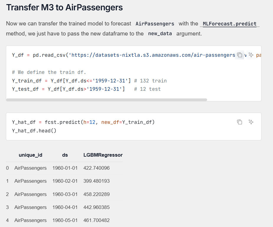
Now, a new product (e.g., a new beverage SKU) is launched in 2025. We only have 3 months of data — clearly not enough to train a new model. Instead, we use the pretrained global model directly and define the new_product data in the new_df argument in predict()call.

new_product = pd.DataFrame({
    'unique_id': 'new_beverage',
    'ds': pd.date_range('2025-01-01', '2025-03-01', freq='MS'),
    'y': [120, 135, 150]
})

# Zero-shot forecast by declaring the new product data in new_df
preds = fcst_global.predict(h=6, new_df=new_product)

Within milliseconds, we get forecasts for April–September 2025 — using a model that never saw this SKU before. By reusing a pretrained global model, transfer learning injects cross-series knowledge — seasonality, promotion response, and trend dynamics — into a new SKU’s forecast, producing reliable zero-shot predictions from only a few months of history. This materially reduces cold-start risk and deployment latency, yielding immediate, business-actionable forecasts that can be further improved through few-shot fine-tuning as real sales accrue.

4. Tackling the Core Questions

Every data scientist in production faces these — here are evidence-based answers:

Q1. Should we retrain every month?

No. Retrain only when drift is detected or significant pattern shifts occur.
Monthly updates can be handled efficiently via update().
Retraining every month adds cost but minimal accuracy gain.

Q2. How to handle new product launches with little history?

Use transfer learning.
Leverage pretrained models trained on thousands of similar products to forecast new SKUs zero-shot.
This drastically reduces cold-start time and aligns inventory early in the lifecycle.

Q3. How do we ensure explainability?

Tree-based models (XGBoost, LightGBM, RF) offer SHAP-based interpretability. By examining feature importance (lags, month, exogenous factors), data scientists can explain:

• Why certain months drive peaks (seasonality),
• How price/promotion covariates affect demand.

This builds business trust — crucial for adoption.

Q4. What’s the optimal strategy for production deployment?

This hybrid approach maximizes ROI and minimizes technical debt.

Closing Thoughts

Forecasting in this age is not about picking the “best” model — it’s about building a system that learns continuously, scales efficiently, and adapts gracefully.

Nixtla’s MLForecast embodies this philosophy:

• update() bridges data continuity with operational speed.
• Transfer learning solves the cold-start and scalability challenge.
• Global models unify forecasting across thousands of time series.

For researchers, it provides a new framework for large-scale empirical forecasting. For industry, it delivers the agility needed for modern retail supply chains.

The intersection of these two worlds — science and production — is where MLForecast truly shines.

Acknowledgement:

1. Nixtla’s MLForecast Documentation
2. García, D. et al. (2023). Global Models for Time Series Forecasting: Principles and Practice, Nixtla Research.
3. Hyndman, R.J., Athanasopoulos, G., Garza, A., Challu, C., Mergenthaler, M., & Olivares, K.G. (2024). Forecasting: Principles and Practice, the Pythonic Way. OTexts: Melbourne, Australia.
4. Can Machine Learning Outperform Statistical Models for Time Series Forecasting? — Towards AI Medium Blog
5. How to MLForecast your Time Series Data! — Level Up Coding Medium Blog

A Practical Guide to Incremental Updates and Transfer Learning for Scalable New-Product Forecasting… was originally published in Level Up Coding on Medium, where people are continuing the conversation by highlighting and responding to this story.

This content originally appeared on Level Up Coding – Medium and was authored by Satyajit Chaudhuri