This content originally appeared on HackerNoon and was authored by Oligopoly
:::info Authors:
(1) Enis Chenchene, Department of Mathematics and Scientific Computing, University of Graz;
(2) Hui Huang, Department of Mathematics and Scientific Computing, University of Graz;
(3) Jinniao Qiu, Department of Mathematics and Statistics, University of Calgary.
:::
Table of Links
2.1 Quantitative Laplace principle
2.2 Global convergence in mean-field law
3 Numerical experiments and 3.1 One-dimensional illustrative example
3.2 Nonlinear oligopoly games with several goods
4 Conclusion, Acknowledgments, Appendix, and References
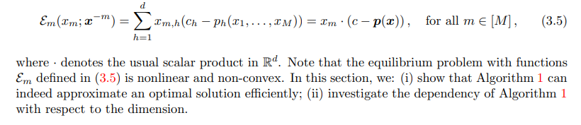
3.2 Nonlinear oligopoly games with several goods
\
\
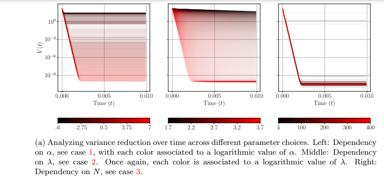
\ Figure 2: Studying the dependence of Algorithm 1 with respect to the algorithm’s parameters to solve (3.5).
\ of good produced, namely
\
\ 3.2.1 Experimental setup
\
\ 3.2.2 Results and discussio
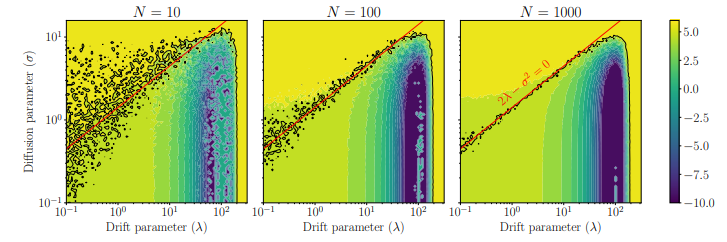
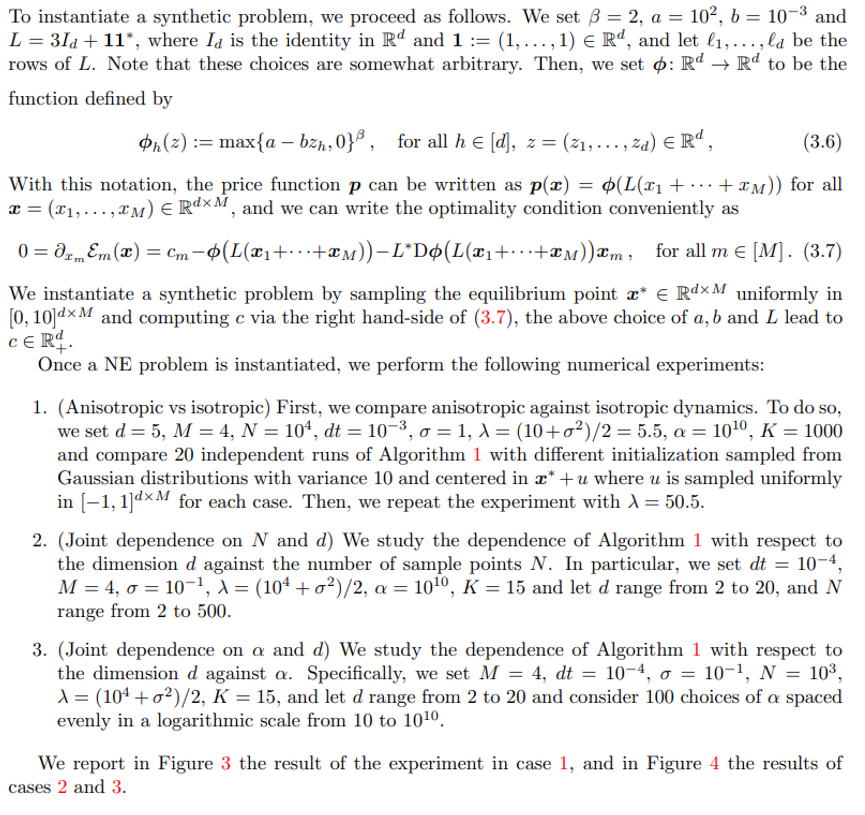
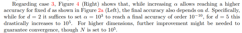
\ In Figure 3, which shows the results corresponding to the experiment in case 1, as observed for instance in [28], we see that the anisotropic case does indeed show a faster convergence rate especially in the initial iterations and for λ which is of the order of σ 2 . If λ increases, though, we see no significant differences in the convergence behavior of anisotropic or isotropic dynamics, both for the residual and for the variance decrease.
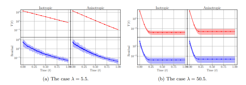
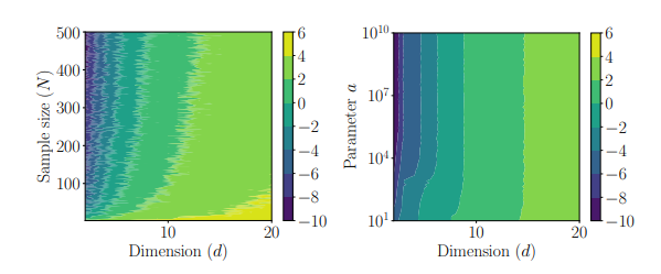
\ Figure 4 shows the results of the comparisons in cases 3 and 2. Regarding case 2, we can see that indeed as the dimension increases, we need exponentially many particles (quantified by N) to reach high accuracy of order 10−9 . This indicates that Algorithm 1, while being quite reliable, and sometimes the only available solver for low-dimensional problems, might need further improvement in high-dimensional settings.
\
\
\
\
:::info This paper is available on arxiv under CC BY 4.0 DEED license.
:::
\
This content originally appeared on HackerNoon and was authored by Oligopoly